Display experimental images

The functions: imagesc , imageph , imagebw , imagegb , imagejet , imagehsv , imagehot , imagefl 

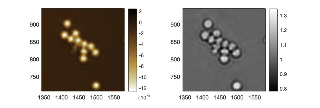
Once the ImageQLSI objects have been created, they contain all the information regarding the QLSI images. In particular, the OPD and intensity images (matrices) can be accessed by writing IM.OPD and IM.T.

The images can be displayed using any standard function of Matlab. We recommend using the native imagesc matlab function, this way:

figure
imagesc(IM.OPD)
set(gca,'DataAspectRatio',[1 1 1]) % avoids image distorsion
colormap(Sepia)
colorbar

To avoid repeating all these code lines each time one wants to display the OPD images, all these code lines have been embeddedd within the imageph function:

figure
imageph(IM.OPD)

Other similar functions are defined, each using a different colorscale, namely

imageX functions for displaying images
Function name	Associated colorscale
`imagegb`	parula
`imageph`	sepia
`imagebw`	gray
`imagejet`	jet
`imagehsv`	hsv
`imagehot`	hot
`imagefl`	invertedGreen()

The dynamicFigure function

dynamicFigure() is a function that can display more than one type of image in one figure (wavefront and intensity for instance). It also enables the navigation thoughout a series of images using the left- and right-arrow keys of the keyboard.

For instance:

dynamicFigure('ph', IM)

displays the OPD image of the IM object. If IM is an array of ImageQLSI objects, then it displays the OPD of the first object, and one can go from one OPD to the following one by using the left and right arrows. This way, all the OPD images of the IM array can be easily visualized.

One can also display more than one image per figure. For instance, to display both wavefront and intensity, the synthax is:

dynamicFigure('ph', IMlist,'bw', {IMlist.T})
linkAxes

Don’t forget the braces when calling the property of the object. The keywork 'bw' just means here display in gray scale. The command linkAxes is optional. It links the two images so that any rescaling of the images using the zoom tool applies to both images.

There is no limit in the number of images that can be displayed. On can for instance write:

dynamicFigure('ph', IMlist,'bw', {IMlist.T},'bw', {IMlist.DWx},'bw', {IMlist.DWy})
linkAxes

to display the wavefront gradients as well.

To display a figure full screen, append the command:

fullscreen

To display a figure over the full screen width, append the command:

fullwidth

One can also use this function to display interferograms (main and reference):

dynamicFigure('bw', {Itf.Itf}, 'bw', {Itf.Ref.Itf})
fullscreen

One can add the "titles" keyword to enter titles to be displayed on top of each image:

dynamicFigure('gb',IM,'gb',{IM.DWx},'gb',{IM.DWy}, ...
     "titles",{'OPD','DWx','DWy'})
linkAxes

Note

Importantly, this function also works if IM or Itf is an object array. In this case, the first object of the series is primarily displayed, and then, by pressing the right-arrow or left-arrow keys, one can navigate to the next or previous images.

The figure method

The classes ImageQLSI and ImageEM have a common method called figure, aimed to display the wavefront and intensity images of an ImageQLSI object, or object array, on a GUI. The possible synthaxes are:

IM.figure()

or

app = IM.figure();

It displays an advanced Matlab GUI where the wavefront and intensity images are displayed, along with a set of tools, for data processing and rendering. A full section is dedicated to this important feature of PhaseLAB. See Section The GUI of PhaseLAB.

The opendx method

The classes ImageQLSI and ImageEM have a common method called opendx, aimed to display the wavefront and intensity images with a 3D rendering. The synthax is:

IM.opendx()
IM.opendx(Name, Value)

Here is an example of 3D rendering using the opendx method, compared with the rendering of the imageph function:

For more information on the opendx method, see The opendx method section.

Color scales

All the native color scales of Matlab can naturally be used when displaying PhaseLAB images. Also, in the /src/colorMaps folder, there are predefined colormaps. To display them, just execute the following command, and a window will appear with all of them:

displayColormaps()

To use any of them, use the colormap command:

colormap(Pradeep)

where the input is simply the name of the desired color map.

Color scale generator

colorMapGenerator is PhaseLAB function aimed to easily create user-designed color maps. Here is an example:

colorList = ["000000";"560000";"AD3200";"FF8B00";"FFD900";"FFFF5B";"FFFFFF"];
% colorList = ["ffffff";"d9d1a7";"b4913e";"805b28";"492d15";"000000"];
% colorList = ["100080";"6500dc";"9a00c4";"d21536";"ff8000";"ffe700";"ffffff"];

posList = [0, 17, 33, 50, 66, 84, 100];

colMap = colorScaleGenerator(colorList,posList,256);

figure
imagegb(meshgrid(1:1024,1:100))
colormap(colMap)

In line 1, a series of 7 colors is stored in a string array, in HEX format.

Line 2 and 3 are other examples of color arrays

Line 5 defines a vector that gathers the positions of the color along an axis going from 0 to 100.

Line 7 uses the colorScaleGenerator function to create a 256x3 color matrix, in the format of a colormap variable to be used as an in put of the colormap function, as shown in line 11.