The ImageQLSI class
ImageQLSI is a handle class.
Properties
name |
type |
default |
description |
|---|---|---|---|
|
Microscope |
Microscope object |
|
|
Illumination |
Illumination object |
|
|
char |
Any comment on the image |
name |
type |
description |
|---|---|---|
|
double array |
Intensity image |
|
double array |
OPD image |
|
double array |
OPD gradient along x |
|
double array |
OPD gradient along y |
name |
type |
description |
|---|---|---|
|
double array |
OPD in nm |
|
double array |
Phase image |
|
double |
Number of columns |
|
double |
Number of rows |
Constructor
Constructor
Synthax
obj = ImageQLSI()
obj = ImageQLSI(n)
obj = ImageQLSI(INT,OPD, MI, IL)
obj = ImageQLSI(obj0)
obj = ImageQLSI(___,Name,Value)
obj = ImageQLSI() creates an empty ImageQLSI object.
objList = ImageQLSI(n) create a n-vector objList of empty ImageQLSI objects.
obj = ImageQLSI(obj0) creates a ImageQLSI object obj from an ImageEM object obj0.
obj = ImageQLSI(INT, OPD, MI, IL) creates an ImageQLSI object, INT defining the intensity image, OPD the optical path difference, MI the microscope and IL the illumination.
INT an OPD can be either a matrix, or a file name (char) containing the data. MI is a Microscope object. IL is an Illumination object.
ImageQLSI accepts Name-Value options.
Examples
**Build an ImageQLSI object by importing data*
T = readMatrix('data/T.txt');
W = readMatrix('data/W.txt');

MI = Microscope(100);         % creates a microscope with 100x magnification
IL = Illumintation (530e-9);  % creates an illumination at lambda = 530 nm

IM = ImageQLSI(T, W, MI, IL); % creates the ImageQLSI object
Name-value arguments
Note
Specify optional pairs of arguments as Name1 = Value1, ..., NameN = ValueN, where Name is the argument name and Value is the corresponding value. Name-value arguments must appear after other arguments, but the order of the pairs does not matter.
Example: ImageQLSI(___,'remotePath','images/data')
remotePathWhen working with a long vector of ImageQLSI objects, one can save RAM memory by storing the
TandOPDmatrices on the hard disk drive, when creating the objects. For this purpose, specify the folder to store these data.FileNameThe
remotePathoption has to be used in conjonction with theFileNameoption, specifying the prefix of the files saved of the computer.
ImageQLSI methods
alpha_ImageProfile
Return the polarisability, optical volume and dry mass of small objects.
Synthax
% prototype
params = obj.alpha_ImageProfile(Name,Value);

% examples
params = obj.alpha_ImageProfile();
params = obj.alpha_ImageProfile('nmax', 100, 'nBkg', 4);
Description
This method of the ImageEM and ImageQLSI classes returns the polarisability, OV and DM of small objects, using a radial profile method. The algorithm involves a sum of the pixels on a circular area. The method opens a window with the image. First, click on the OPD image to zoom in on the particle of interest, and press ‘z’ when the zoom is correct. Second, click on the center of the particle. A new figure will show up, plotting the pixel summation as a function of the radius of the circular area, from 0 to 100 px. Finally, click two times on the graph to define the range of values corresponding to a proper convergence of the integration. In practice, the line shape should feature a plateau, and the user should click at the beginning and at the end of the plateau. For instance, in this example, the user could click on \(x=18\) and \(x=40\):

Finally, the values of polarisability, and optical volume are returned as a structure, containing the fields alpha, OV and OVw. OVw is the weighted optical volume as defined in Ref. 1.
- 1
Biomass measurements of single neurites in vitro using optical wavefront microscopy, L. Durdevic, A. Resano Gines, A. Roueff, G. Blivet, G. Baffou, Biomedical Optics Express 13, 6550-6560 (2022)
Name-Value inputs
Several Name-Value inputs can be used to adjust the way the procedure works:
'nmax', default value:40Maximum radius of the integration area.
'nBkg', default value:3Width of the boundary considered to calculate the zero value of the background.
'NNP', default value:1Number of particles to be clicked on the image. The procedure stops after
Nparticles are processed, and the returned data is an array of values.'zoom', default value:trueEnables the user to first zoom before clicking on the particle
'step', default value:1The integration as a function of the radius will be calculated only every
Npixels, whereNis the step value. Specifying a value larger than 1 can make the processing faster.'keepPoint', default value:falseKeeps the same clicking point from one image to another. It can save time if many images need to be processed, and if the NP does not move from one image to another.
'display', default value:falseDisplays the results of all the measurements in a single graph. Makes sense only if multiple measurements are made within a single call of the function.
binning
Performs 2x2 or 3x3 pixel binning of the images of the ImageQLSI object.
Synthax
obj.binning()
obj.binning(n)
obj2 = obj.binning(___);
Description
obj can be a vector of ImageQLSI objects. In that case, the treatment will be performed on all the objects of the list.
obj.binning() performs, by default, a 3x3 binning of the images of obj.
obj.binning(n) performs, \(n\times n\) binning of the images of obj. Only works with n = 2 or n = 3.
If an output argument is specified, obj is not modified, but duplicated.
crop
Crop the images of the object.
Synthax
obj.crop()
obj.crop(Name, Value)
objList.crop(___)
obj2 = obj.crop(___);
[obj2, params] = obj.crop(___);
Description
obj.crop() crops the \(E\) fields of the object and of the Ref object, identically. A figure window opens, inviting the user to click on the image to define a square area centered in the middle of the image.
Objects vectors can also be used with this method. The transformation applies then to all the objects of the vector.
If an output is used, obj2, then the object is not modified, but duplicated.
If a second output is specified, then the crop parameters are returned as a 4-vector params = [x1, x2, y1, y2];
Name-value arguments
Note
Specify optional pairs of arguments as Name1 = Value1, ..., NameN = ValueN, where Name is the argument name and Value is the corresponding value. Name-value arguments must appear after other arguments, but the order of the pairs does not matter.
Example:
obj.crop(___,'Center','Manual','Size',300)
'Center'With
crop(___,'Center','Manual'), the user has to first click on the center of the reference area. If the argument is set to'Auto', then this step is skipped, and the center is automatically set to the center of the image. Also, the user can indicate the coordinates of the center usingcrop(___,'Center',[x_c, y_c]).'Size'With
crop(___,'Size','Manual'), once the center is defined (either manually or automatically), the user has to click on the figure to define the shape of the area, around the center point. The user can also indicate the dimensions of the reference area usingcrop(___,'Size',Npx)for a square area, orcrop(___,'Size',[Nx, Ny])for a rectangular area.'twoPoints'Instead of using the
'Center'and'Size'keywords, one can also click on two opposite corners of the reference area, usingcrop(___,'twoPoints',true).'params'One can also direclty write the coordinates of the crops, using
crop(___,'params', [x1, x2, y1, y2]). In this case, no figure opens.
Here is an example of a code that crops a first object manually, and applies automatically the same crop to a second object:
[IMc(1) params] = IM(1).crop('Center', 'Manual', 'Size', 'Manual');
IMc(2) = IM(2).crop('params', params);
Note that this code is equivalent to:
IMc = IM.crop('Center', 'Manual', 'Size', 'Manual');
dmd
Return the dry mass density (DMD) image.
Synthax
val = obj.dmd();
Description
val is the DMD image, in pg/µm2. This function actually just consists of multiplying the OPD in [nm] by 5.56e-3.
download
Import on the RAM of the computer an object that is in ‘remote’ mode.
Synthax
obj2 = obj.download();
Description
Import on the RAM of the computer an object that is in ‘remote’ mode, i.e., where the T and OPD properties are stored in the hard disk drive. This happens when creating an ImageQLSI object using obj = QLSIprocess(___, 'remote', true);.
DWnorm
Returns the norm of the gradient of the OPD image of the ImageQLSI object.
Synthax
val = obj.DWnorm()
Returns the norm of the gradient image, computed from the two gradient images DWx and DWy.
Caution
When accessing the image gradients by writing IM.DWx or IM.DWy, matlab checks whether these matrices exist in the object. They exist if the option saveGradients was set to true when creating the object IM using the QLSIprocess method (of the class interfero).
IM = Itf.QLSIprocess(IL, 'saveGradients', true)
If this option was not used, then Matlab computes the gradients from the OPD image, each time the gradients are called. This latter approach is not recommended. If the gradients need to be used for any reason after the ImageQLSI objects are created, we recommend using the 'saveGradients' option when calling the QLSIprocess method.
dxSize
Return the dexel size.
Synthax
val = obj.dxSize();
Description
Returns the dexel size (i.e. the camera pixel size), val = obj.Microscope.CGcam.dxSize;.
Note
This method returns the effective dexel size, which is not necessarily the actual dexel size of the camera sensor. When there is a RL, applying a zoom \(Z\) to the system, the {RL, camera} system is equivalent to a single camera with a dexel size divided by the zoom. This method returns the dexel size of this equivalent camera, called the effective dexel size.
D2Wnorm
Return the second derivative (Laplacian) of the OPD image of the ImageQLSI object.
Synthax
val = obj.D2Wnorm()
Returns the second derivative (Laplacian) of the OPD image of the ImageQLSI object, computed from the two gradient images DWx and DWy.
Caution
When accessing the image gradients by writing IM.DWx or IM.DWy, matlab checks whether these matrices exist in the object. They exist if the option saveGradients was set to true when creating the object IM using the QLSIprocess method (of the class interfero).
IM = Itf.QLSIprocess(IL, 'saveGradients', true)
If this option was not used, then Matlab computes the gradients from the OPD image, each time the gradients are called. This latter approach is not recommended. If the gradients need to be used for any reason after the ImageQLSI objects are created, we recommend using the 'saveGradients' option when calling the QLSIprocess method.
figure
Display the PhaseLAB GUI
Synthax
obj.figure()
app = obj.figure();
Description
This method displays the images of the obj within the GUI (graphical user interface) of PhaseLAB. See the GUI of PhaseLAB section for details.
flatten
Flatten the background of the OPD image.
The flatten method corrects any artefactual image distorsion, which comes for instance from a mismatch between the reference image and the object image. To flatten the image, this method either removes a blurred image to the image ('Gaussian' mode) or computes the low-order moments of the images and subtract them.
Synthax
% general form
obj.flatten()
obj.flatten(method)
obj.flatten(___, Name, Value)
objList.flatten(___)
obj2 = obj.flatten(___);

% examples
obj.flatten('Zernike')
obj.flatten('Legendre', 'mnax', 3, 'threshold', 1.2);
obj.flatten('Chebyshev', 'kind', 1, 'mnax', 3, 'display', true)
obj.flatten('Gaussian', 'nGauss', 100);
obj.flatten('Legendre', 'nmax', 4, 'mask', booleanMatrix);
obj.flatten('Legendre', 'nmax', 4,  'threshold', 1.2, 'nGauss', 10, 'cut', 0.5, 'invert', true);
obj.flatten('Legendre', 'nmax', 4,  'params', params);
Description
obj.flatten() removes the tilt and coma aberration of the image, by a smoothed image subtraction, with a smoothing parameter nGauss = 100.
obj.flatten(method) removes the tilt and coma aberration of the image, where the image moments belong to a specific class of polynomials. The possible values of the method input are 'Waves', 'Zernike', 'Chebyshev', 'Hermite', 'Legendre'. This is also the option 'Gaussian'. In this latter case, not moment is calculated, and the background correction is obtained by a subtration of a blurred image.
obj.flatten(___, Name, Value) enables the use of optional inputs, defined by keywords 'Name'.
The possibles Names are:
'nmax'Tells until which order the image moments are calculated (inactive if
method = 'Gaussian'). For instance,obj.flatten('Legendre', 'nmax', 2)
removes all the \((n,m)\) Legendre moments from the image such that \(n+m\le n_\mathrm{max}=2\), i.e., (0, 0), (1, 0), (0, 1), (1, 1), (2, 0), (0, 2). Here is a repesentation of the Legendre polynomials. Alternatively,
nmaxcanbe a 2-vector representing the maximum values of \(n\) and \(m\):obj.flatten('Legendre', 'nmax', [2,2])
removes all the \((n,m)\) Legendre moments from the image such that \(n\le n_\mathrm{max}=2\) and \(m\le m_\mathrm{max}=2\), i.e., (0, 0), (1, 0), (0, 1), (1, 1), (2, 0), (0, 2), (2, 1), (1, 2), (2, 2).

obj.flatten('Zernike', 'nmax', 2)
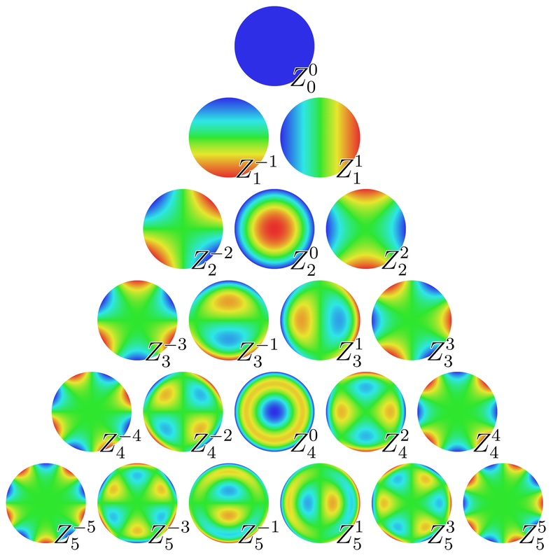
removes all the \((n,m)\) Zernike moments from the image up to \(n=n_mathrm{max}=2\), i.e., (0, 0), (1, -1), (1, 1), (2, -2), (2, 0), (2, 2). Here is a representation of the Zernike polynomials.
'kind'Used when using the Chebyshev method. Tells whether Chebyshev polynoms of the 1st or 2nd kind should be used.
'nGauss'Used when using the Gaussian method. The value is the parameter used with the imgaussfilt function that makes the blurred image to be subtracted. The larger this value, the lesser the flatten effect.
'nGauss = 100'is the default value, and a good starting value.'threshold'It is common to observe thick objects within the field of view of the microscope, like eukaryotic cells. Such objects would contribute to the moment computation while they should not. The moment should only consider distorsion of the background. The flatten function can be used to compute the moments only stemming from the background of the image. For this purpose, the code has to determine which part of the image is the background (or reciprocally, which part of the image is the object). For this purpose, a segmentation procedure is used, optimized for the study of eukaryotic cells. The procedure involves a free parameter that is specified using this
'threshold'parameter. A value a 1 is a good starting value.'mask'For some samples, the automatic segmentation procudure that is used when setting a value to
thresholdmay be uneffective. In this case, one can specify a mask, as a matrix of the same size as the image, with 0 and 1 values, where the 1 values define to the background area. This mask is to be built by the user itself in the main PhaseLAB file before calling the function flatten. See the Background flattening tutorial for more information on how to create a mask, and use thethreshold,nGauss,cut, andinvertparameters.'display'Equals true or false. If true, the segmentation of the background is displayed, as a means to visually check it is effective.
fliplr
Flips the images of the object about the vertical axis (flips left-right).
Synthax
obj.fliplr();
objList.fliplr();
obj2 = obj.fliplr();
Description
ImageQLSI objects vectors can also be used with this method. The transformation applies then to all the objects of the vector.
If an output obj2 is used, then the object is not modified, and duplicated.
flipud
Flips the images of the object about the horizontal axis (flips up-down).
Synthax
obj.flipud();
objList.flipud();
obj2 = obj.flipud();
Description
ImageQLSI objects vectors can also be used with this method. The transformation applies then to all the objects of the vector.
If an output obj2 is used, then the object is not modified, and duplicated.
highPassFilter
Applies a high-pass filter on the spatial frequencies of the image, as a means to remove the lwo frequencies and highlight the details.
Synthax
obj.highPassFilter()
obj.highPassFilter(n)
obj2 = obj.highPassFilter(___)
objList.highPassFilter(___)
objList2 = objList.highPassFilter(___)
Description
obj.highPassFilter() applies a high-pass filter on the spatial frequencies of the OPD image, as a means to remove the low frequencies and highlight the details. It actually removes a Gaussian-blurring of the image from the image. For this purpose, it uses the imgaussfilt function with, by default, sigma = 10.
obj.highPassFilter(n) applies a high-pass filter on the spatial frequencies of the image. n is the sigma parameter of the imgaussfilt function. The larger n, the flatter the OPD image looks.
ImageQLSI objects vectors can also be used with this method. The transformation applies then to all the objects of the vector.
If an output is used, obj2, then the object is not modified, and duplicated.
imageHSV
display a mix of the T an OPD images according to a HSV colorscale pattern.
Synthax
imageHSV(obj);
Description
The imageHSV method displays a mix of the intensity an OPD images according to a HSV pattern. Just like the RVB coding, HSV coding codes any color with 3 numbers:
H means Hue and represents the color on a chromatic circle
S means Saturation and tells if the colors are vivid or pale.
V means Value and tells if the color is bright or dark.
Here is a picture that explains the HSV color coding:

Example
The imageHSV method assigns the OPD image to the Hue (the colorscale), and the intensity image to the Saturation (this way, areas with low intensity appear dark), and keeping the Value to 1.
lambda
Return the wavelength of the illumination.
Synthax
val = obj.lambda();
Description
This method returns the wavelength of the illumination used to acquire the image, val = obj.Illumination.lambda;.
level0
Offset the OPD image to adjust the background value to zero.
Synthax
obj.level0()
obj.level0(Name, Value)
objList.level0(___)
obj2 = obj.level0(___);
[obj2, params] = obj.level0(___);
Description
obj.level0() adjusts the offset of the image. More precisely. This method asks for an area on the image, the average value of which should be zero. The method applies an offset to the whole image to satifies this condition. Many options can be specified to tell how this area is selected. See below.
Object vectors can also be used with this method. The transformation applies then to all the objects of the vector, with the same reference area.
If an output is used, obj2, then the object is not modified, but duplicated.
If a second output is specified, then the area parameters are returned as a 4-vector params = [x1, x2, y1, y2];
Name-value arguments
Note
Specify optional pairs of arguments as Name1 = Value1, ..., NameN = ValueN, where Name is the argument name and Value is the corresponding value. Name-value arguments must appear after other arguments, but the order of the pairs does not matter.
Example:
obj.level0(___,'Center','Manual','Size',300)
'Center'With
level0(___,'Center','Manual'), the user has to first click on the center of the reference area. If the argument is set to'Auto', then this step is skipped, and the center is automatically set to the center of the image. Also, the user can indicate the coordinates of the center usinglevel0(___,'Center',[x_c, y_c]).'Size'With
level0(___,'Size','Manual'), once the center is defined (either manually or automatically), the user has to click on the figure to define the shape of the area, around the center point. The user can also indicate the dimensions of the reference area usinglevel0(___,'Size',Npx)for a square area, orlevel0(___,'Size',[Nx, Ny])for a rectangular area.'twoPoints'Instead of using the
'Center'and'Size'keywords, one can also click on two opposite corners of the reference area, usinglevel0(___,'twoPoints',true).'params'One can also direclty write the coordinates of the area, using
level0(___,'params', [x1, x2, y1, y2]). In this case, no figure opens.
Here is an example of a code that manually ajusts the offset of a first object, and applies automatically the same adjustment to a second object:
[IMc(1) params] = IM(1).level0('Center', 'Manual', 'Size', 'Manual');
IMc(2) = IM(2).level0('params', params);
Note that this code is equivalent to:
IMc = IM.level0('Center', 'Manual', 'Size', 'Manual');
MakeMoviedx
Make a movie from a series of image objects
Synthax
% prototypes
objList.makeMoviedx(videoName)
objList.makeMoviedx(videoName, Name, Value)

% examples
objList.makeMoviedx('movie/bacteria.avi')
objList.makeMoviedx('movie/bacteria.avi', )
objList.makeMoviedx('movie/bacteria.avi','theta',0,'phi',0,'rate',2,'zrange',[-10 10])
Description
The MakeMoviedx method creates an .avi movie from an ImageEM or ImageQLSI object array. Two inputs are required, the image object array IM and the path/name of the movie file to be created videoname. It calls the method opendx, from the same class.
Many Name-value options can be specified to change the rendering.
'persp'(default:1)With
'persp'set to1, the video uses theopendxmethod to create a nice 3D rendering of the image. Set this option to0to cancel this effect.'phi'(default:45) and'theta'(default:45)Position of the camera in
(theta, phi).(0,0)corresponds to the top view.'ampl'(default:3)sets the magnitude of the 3D visual topography
'zrange'2-vector setting the limits of the \(z\) axis.
'colorMap'(default:Parula)Color map.
'title'Title to display on the movie, if any.
'factor'(default:1)Correction factor to the OPD, for instance 5.55e-3 to convert the OPD into DM.
'label'(default:'Optical path difference (nm)')Label to put on the color scale.
'imType'(default:'OPD')Cell array of the images of the object to be displayed within the figure of the movie, side by side:
'OPD','T','DWx','DWy','Ph'.'axisDisplay'(default:true)Display the axes or not.
'rate'(default:25)Video rate in frames per second.
'frameTime'(default:[])Time between successive frames. If specified, the time is displayed on each frame.
'timeUnit'(default:s)Unit of the time to be displayed. Can be
's','min'or'h'.'timeFontSize'(default:[])Set the font size displayed on the movie.
'timeFontColor'(default:[0, 0, 0])Set the color of the displayed time label. By default it is black, but depending on the colormap of the image, it may be necessary to use a brighter color. White is
[1, 1, 1].'timeSize'If the default size is not appropriate, choose a specific one using this option.
16can be a good starting value.
mean
Average the OPD and T images of a list of ImageQLSI objects.
opendx
Display a 3D rendering of the image
Synthax
% prototypes
opendx(obj)
opendx(obj, Name, Value)

% examples
opendx(IM)
objList.makeMoviedx(IM, 'theta', 10, 'phi', 30, 'zrange', [-10 120]*1e-9, 'ampl', 4)
Description
The opendx method diplays images from ImageEM or ImageQLSI objects with a nice 3D rendering.
Many Name-value options can be specified to change the rendering.
'persp'(default:1)With
'persp'set to1, the video uses theopendxmethod to create a nnince 3D rendering of the image. Set this option to0to cancel this effect.'phi'(default:45) and'theta'(default:45)Position of the camera in \((\theta, \phi)\)
'ampl'(default:3)sets the magnitude of the 3D relief
'zrange'2-vector setting the limits of the z axis.
'colorMap'(default:parula)Color map.
'title'Title to display on the movie, if any.
'factor'(default:1)Correction factor to the OPD, for instance 5.55e-3 to convert the OPD into DM.
'label'(default:'Optical path difference (nm)')Label to put on the color scale.
'imType'(default:'OPD')Cell array of the properties of the object to be displayed:
'OPD','T','DWx','DWy','Ph'.'axisDisplay'(default:true)Display the axes or not.
overview
Display all the images of an object array in a single figure
Synthax
objList.overview();
objList.overview('types', typeList)
Description
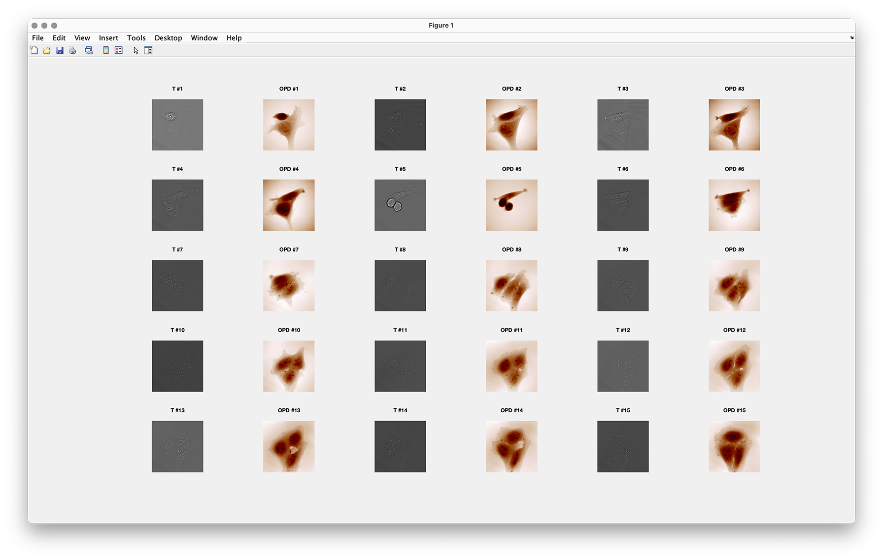
This method displays all the images of an object array in a single figure. Here is an example of what it gives with an array of 15 objects:
PDCM
Computes the PDCM (phase derivatives closure map) of the OPD image.
Synthax
val = obj.PDCM()
Description
obj.PDCM() computes the PDCM (phase derivatives closure map) of the OPD image, as introduced by J. Rizzi et al. 2. It is defines as
Caution
This function needs to access the IM.DWx and IM.DWy properties. When accessing the image gradients by writing IM.DWx or IM.DWy, matlab checks whether these matrices exist in the object. They exist if the option saveGradients was set to true when creating the object IM using the QLSIprocess method (of the class interfero).
IM = Itf.QLSIprocess(IL, 'saveGradients', true)
If this option was not used, then Matlab computes the gradients from the OPD image, each time the gradients are called. This latter approach is not recommended. If the gradients need to be used for any reason after the ImageQLSI objects are created, we recommend using the 'saveGradients' option when calling the QLSIprocess method.
- 2
Opt. Express 21, 17340 (2013)
propagation
Apply a variation of the microscope focus on the images.
Synthax
% general form
obj.propagation(z)
objList.propagation(z)
obj2 = obj.propagation(z);

% examples
obj.propagation(-1e-6)
obj2 = obj.propagation(0.2e-6);
Description
obj.propagation(z) computes the new T and OPD images when a variation z of the focus of the microscope is numerically applied.
Objects vectors can also be used with this method. The transformation applies then to all the objects of the vector.
If an output obj2 is used, obj2 = obj.propagation(z), then the object is not modified, and is duplicated.
Example
Numerical refocusing
Code to numerically modify the focus of the image
%% Code that imports one experimental image (of long Geobacillus bacteria)
%% and creates a series of images at different focuses from this single image

ME = Medium('water','glass');
OB = Objective(100,0.7,'Olympus');
MI = Microscope(OB,200,'sC8-944','PhaseLIVE');
lambda = 531e-9;
IL = Illumination(lambda,ME);

%% IMPORT THE IMAGES
folder = 'GeobLongFilaments';
Im = importItfRef(folder,MI);

%% INTERFEROGRAM PROCESSING
IM = Im.QLSIprocess(IL);

%% list of defocus values in µm
zList = -20:10;
No = length(zList);

IMlist = ImageQLSI(No);

for io = 1:No
    IMlist(io) = copy(IM(1));
    IMlist(io) = IMlist(io).propagation(zList(io)*1e-6);
    IMlist(io).comment = [num2str(zList(io)) ' µm'];
end

% select the area supposed to correspond to a zero wavfront value
IMlist.level0(Center="Manual", Size="Manual");

% crop the image
IMlist.crop(Size=2000);

% build a movie from the series of images:
IMlist.makeMoviedx('/Users/perseus/Documents/im.avi', ...
    persp=0,theta=0, phi=0, ...
    zrange = [-80, 100])
pxSize
Return the image pixel size at the sample plane.
Synthax
val = obj.pxSize();
Description
Returns the pixel size at the sample plane.
rot90
Rotate the images of the object by multiples of 90°.
Synthax
obj.rot90();
obj.rot90(k);
objList.rot90(___);
obj2 = obj.rot90(___);
Description
obj.rot90() rotates the images of the object by 90°, counterclockwise.
obj.rot90(k) rotates the images of the object by \(k\times90°\), counterclockwise. k must be an integer and can be negative.
ImageQLSI objects vectors can also be used with this method. The transformation applies then to all the objects of the vector.
If an output obj2 is used, then the object is not modified, and duplicated.
Rytov
Return the Rytov image.
Synthax
val = obj.Rytov();
Description
Method that returns the Rytov image, defined by 3
where \(\lambda\) is the wavelength, \(n\) the refractive index of the surrounding medium, \(T\) the intensity image and \(\varphi\) the phase image.
save
Export the T and OPD images as jpg and txt files.
Synthax
% general patterns
obj.save(folder)
obj.save(folder, Names)

% Examples,
obj.save('savedData', 'T')
obj.save('savedData', 'OPD')
obj.save('savedData', 'T', 'OPD')
obj.save('savedData', 'T', 'OPD', 'DWx', 'DWy', 'Ph')
Description
Export the intensity, wavefront, phase and/or gradient images of the ImageQLSI object into a folder, as .txt and .jpg files. To indicate which images are saved, a list a keywords has to be indicated as separated arguments, corresponding to the names of the properies.
sizeof
sizeof
Returns the size of the object in Kb.
Synthax
obj.sizeof()
val = obj.sizeof();
Description
Returns or display the size of the object (list) occupied on the hard drive. If not output is specified, it displays the size, in Mb, or Kb, in the command window. Otherwise, it returns the size in bytes.
smooth
Applies a low-pass filter on the spatial frequencies of the image, as a means to blur the image.
Synthax
obj.smooth()
obj.smooth(n)
obj2 = obj.smooth(___)
objList.smooth(___)
objList2 = objList.smooth(___)
Description
obj.smooth() applies a low-pass filter on the spatial frequencies of the OPD image, as a means to remove the high frequencies and blur the OPD image. It actually simply applies a Gaussian-blurring on the OPD image using the imgaussfilt function with, by default, sigma = 10.
obj.smooth(n) applies a low-pass filter on the spatial frequencies of the image. n is the sigma parameter of the imgaussfilt function. The larger n, the flatter the OPD image look.
ImageQLSI objects vectors can also be used with this method. The transformation applies then to all the objects of the vector.
If an output is used, obj2, then the object is not modified, and is duplicated.
square
Transforms rectangle images to square images by cropping.
Synthax
obj.square()
objList.square(___)
obj2 = obj.square(___)
Description
obj.square() crops the images of the ImageQLSI object so that they are square. To define the size of the square, the smallest image dimension is considered (min([obj.Nx, obj.Ny])).
ImageQLSI objects vectors can also be used with this method. The transformation applies then to all the objects of the vector.
If an output is specified, obj2, then the object is not modified, but duplicated.
TMPprocess
Computes a temperature image from a wavefront image.
Synthax
objT = obj.TMPprocess(Med)
objT = obj.TMPprocess(Med, Name, Value)
objListT = objList.TMPprocess(___)
[objT, GreenFunction, GreenT_z0] = objList.TMPprocess(___)
Description
obj.TMPprocess() computes the 2D temperature map associated with a wavefront distorsion. See Ref. 3 for more detail.
Objects vectors can also be used with this method. The transformation applies then to all the objects of the vector.
The output objT is an object from the class ImageT.
This method accepts one input parameter, the variable Med from the class MediumT, defining the thermal properties of the surrounding medium (thermal conductivities and dn/dT values). It also accepts Name-value arguments, as listed below.
Optional outputs are the OPD and temperature Green’s functions. They can be reused in subsequent calls of the TMPprocess function to save computation time.
Name-value arguments
Note
Specify optional pairs of arguments as Name1 = Value1, ..., NameN = ValueN, where Name is the argument name and Value is the corresponding value. Name-value arguments must appear after other arguments, but the order of the pairs does not matter.
'g'and'loop'(default values:1and1)For large temperature increases, a non-linear algorithm is required to obtain accurate temperature increase maps, as explained in Ref.5. In that case, the
'g'and'loop'parameters must be specified. Typical values are 0.4 and 10:objT = TMPprocess(Med, 'g', 0.4, 'loop', 10);
Note that
g=1; loop=1corresponds to the linear algorithm.'alpha'(default value:1e-5)This is the Tikhonov parameter.Keeping it at 1e-5 is usually fine. Higher values tend to smooth the image, and underestimate the temperature increase. Smaller values tend to increase the noise on the temperature image.
'smoothing'(default value:0, that is no smoothing)When the OPD image is very noisy, one may want to smooth it. This can be done using the
smoothmethod of the ImageQLSI class, but also using this Name-Value argument here. If different from zero (the default value), this smoothing option applies theimgaussfiltfunction to the OPD image, the value being the parameter of the imgaussfilt function. The smaller the parameter and the stronger the smoothing.'imExpander'(default value:true)This parameter is a boolean. If set to true, it extrapolates the image over a double-size area to avoid artefacts on the boundaries of the reconstructed temperature image. This parameter is true by default, and we recommend to leave it like that, unless the temperature increase is really located at the center of the image.
'T0'Ambient temperature value, set at 22°C by default.
'zT'Height at which the temperature should be computed. 0 by default, i.e. the interface between the two media.
'GreenOPD'Specifies the OPD Green’s function, in case it has aleady been computed before, just to save computation time.
'GreenT_z0'Specifies the temperature Green’s function, in case it has aleady been computed before, just to save computation time.
'GreenT_3D'Specifies the 3D temperature Green’s function, in case it has aleady been computed before, just to save computation time.
- 4
Thermal Imaging of Nanostructures by Quantitative Optical Phase Analysis, G. Baffou et al., ACS Nano 6, 2452 (2012)
- 5
Three-dimensional temperature imaging around a gold microwire, Applied Physics Letters 102, 244103 (2013)
untilt
Removes a tilt on the OPD image.
Synthax
obj.untilt()
obj.untilt(Name, Value)
objList.untilt(___)
obj2 = obj.untilt(___)
Description
obj.untilt() removes any possible tilt of the OPD image by calculating the (1,1) and (1, -1) Zernike moments of the image, and subtracting the corresponding tilts to the image.
By default, the moment are calculated on the whole image. The power of this methods lies on the fact that the moments can also be calculated on any sub-area of the image, if some Name-value arguments are specified (see next section).
ImageQLSI objects vectors can also be used with this method. The transformation applies then to all the objects of the vector.
If an output is used, obj2, then the object is not modified, and is duplicated.
Name-value arguments
Note
Specify optional pairs of arguments as Name1 = Value1, ..., NameN = ValueN, where Name is the argument name and Value is the corresponding value. Name-value arguments must appear after other arguments, but the order of the pairs does not matter.
The Name-Value arguments in the untilt method are used to define how the reference area is chosen. This reference area is the one that will feature a no-tilt when the tilt correction will be applied. When some arguments are set to 'Manual', a figure appears so that the user can select this area, in 1 or 2 clicks.
'Center'With
untilt(___,'Center','Manual'), the user has to first click on the center of the reference area. If the argument is set to'Auto', then this step is skipped, and the center is automatically set to the center of the image. Also, the user can indicate the coordinates of the center:untilt(___,'Center',[x_c, y_c]).'Size'With
untilt(___,'Size','Manual'), once the center is defined (either manually or automatically), the user has to click on the figure to define the shape of the area, around the center point. The user can also indicate the dimensions of the reference area:untilt(___,'Size',Npx)for a square area, oruntilt(___,'Size',[Nx, Ny])for a rectangular area.'twoPoints'Instead of using the
'Center'and'Size'keywords, one can also click on two opposite corners of the reference area, usinguntilt(___,'twoPoints',true).'params'One can also direclty write the coordinates of the bottom-left and top-right corners, using
crop(___,'params', [x1, x2, y1, y2]). In this case, no figure pops up.
write
copy the properties of an ImageQLSI object into another.
Synthax
write(obj, obj_in)
obj.write(obj_in)
Description
The method copies all the properties of obj_in into the prexisting object obj, without creating a new handle.
ZernikeRemove
Removes the Zernike moments of the OPD image of an ImageQLSI object.
Synthax
obj.ZernikeRemove()
obj.ZernikeRemove(n);
obj.ZernikeRemove(n,m,r);
obj2 = obj.ZernikeRemove(___);
Description
obj.ZernikeRemove() removes, by default, the (n, m) = (1, 1) Zernike order from the OPD image of obj.
obj.ZernikeRemove(n); removes all the Zernike orders up to order n. For instance, obj.ZernikeRemove(2) removes the orders \((1,1)\), \((1,-1)\), \((2,-2)\), \((2,0), :math:\) from the OPD image.
In obj.ZernikeRemove(n,m,r);, r is the radius of the disc over which the Zerninke moment is calculated. By default, it is half the size of the image (r = min([obj.Nx, obj.Ny])/2-1).
If an output obj2 is specified, IM is copied. If not, obj is modified.
+
Defines the addition between two ImageQLSI objects: IM1 + IM2.
Synthax
obj = plus(obj1, obj2);
obj = obj1 + obj2;
obj = obj1 + obj2 + ... + objN;
Description
The method overloads the operator + by defining the method plus. It returns a ImageQLSI object with a weighted sum of the two wavefront and intensity images, defined by:
Such a summation makes sense if the different wavefronts are incoherent with each other. If the wavefront originate from a single coherent light source, then the objects should belong to the ImageEM class, which rather deals with electromagnetic fields.
The method also work with several additions at a time: obj = obj1 + obj2 + ... + objN;