The opendx0 function
Synthax
% prototype
opendx0(img, Name, Value)

% examples
opendx0(Im, "persp", 1 ...
'phi', 45, ...
'theta', 45, ...
'ampl', 10, ...
'zrange', [-20 200]*1e-9, ...
'colorMap',  parula, ...
'title', [], ...
'factor', 1, ... % correction factor, for instance 5.55e-3 to convert the OPD color scale into dry mass
'clabel', '', ...
'pxSize', 65e-9, ...
'figTitle', 'OPD [nm]')
Description
opendx0() is a function that display images with a nice 3D rendering, for instance :

Example
In Silico simulation
In Silico simulation
Code that simulates the image of a gold nanoparticle including shot noise
%% code that simulates the image of a gold nanoparticle including shot noise

lambda = 530e-9;            % Illumination wavelength
Npx = 120;                  % Final image with Npx*Npx pixels

% model the setup
ME = Medium('water', 'glass');
OB = Objective(100,1.0,'Olympus');
CGcam = CGcamera('sC8-944');
MI = Microscope(OB,'Olympus',CGcam);
IL = Illumination(lambda,ME);

% model the nanoparticle
radius = 60e-9;             % Nanoparticle radius
DI = Dipole('Au',radius);   % creation of the Dipole object
DI = DI.shine(IL);          % illumination of the dipole

% compute the images
IM0 = imaging(DI,IL,MI,Npx);

% model the experimental interferogram
Itf = CGMinSilico(IM0,'shotNoise',true);

% processing the in Silico images
IM = QLSIprocess(Itf,IL);

% display the theoretical and in Silico images
dynamicFigure('gb',IM0,'gb',IM)
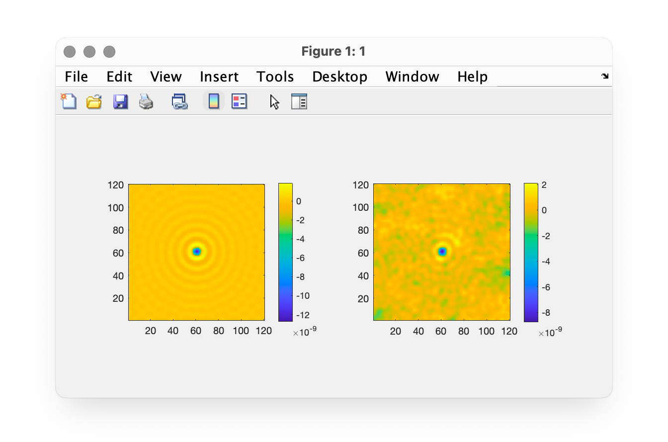
For instance:
1dynamicFigure('ph', IM)
displays the OPD image of the IM object. If IM is an array of ImageQLSI objects, then it displays the OPD of the first object, and one can go from one OPD to the following one by using the left and right arrows. This way, all the OPD images of the IM array can be easily visualized.

One can also display more than one image per figure. For instance, to display both wavefront and intensity, the synthax is:
1dynamicFigure('ph', IMlist,'bw', {IMlist.T})
2linkAxes
Don’t forget the braces when calling the property of the object. The keywork 'bw' just means here display in gray scale. The command linkAxes is optional. It links the two images so that any rescaling of the images using the zoom tool applies to both images.
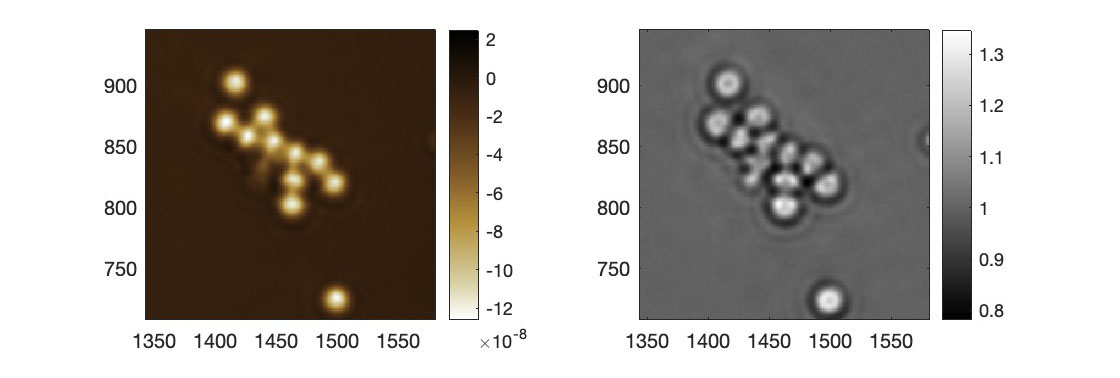
There is no limit in the number of images that can be displayed. On can for instance write:
1dynamicFigure('ph', IMlist,'bw', {IMlist.T},'bw', {IMlist.DWx},'bw', {IMlist.DWy})
2linkAxes

to display the wavefront gradients as well.
To display a figure full screen, append the command:
fullscreen
To display a figure over the full screen width, append the command:
fullwidth
One can also use this function to display interferograms (main and reference):
1dynamicFigure('bw', {Itf.Itf}, 'bw', {Itf.Ref.Itf})
2fullscreen
One can add the "titles" keyword to enter titles to be displayed on top of each image:
1dynamicFigure('gb',IM,'gb',{IM.DWx},'gb',{IM.DWy}, ...
2     "titles",{'OPD','DWx','DWy'})
3linkAxes

Note
Importantly, this function also works if IM or Itf is an object array. In this case, the first object of the series is primarily displayed, and then, by pressing the right-arrow or left-arrow keys, one can navigate to the next or previous images.